TFR and MAB forecast

Overview

After the input data preparation, forecasts for TFR (total fertility rate) and MAB (mean age of the mother at birth) are calculated. In general, the FSO uses the same model structure for both forecasts. However, different model types and parameters can be used for the TFR and MAB forecast.

The FSO model for TFR and MAB consists of three time periods

• trend period: in the FSO model usually a few years (one to five years)
• temporal period: the majority of forecast period (FSO: approximately until 2055)
• constant period: end of the forecast (FSO: from 2056 until 2075)

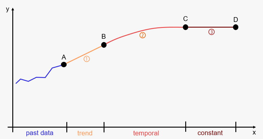
time periods

Trend period

In the original FSO model, for the trend model an ARIMA model is used for the trend period. Depending on the structure of the past TFR and MAB data, the ARIMA forecast is not always stable. Therefore, in propopbirth a linear model can be used as an alternative to the ARIMA model.

If an lm model is used, the window of past years (trend_past) and the proportional amount of past years used to fit the model (trend_prop) can be specified.This allows for weighted or selective emphasis on recent data when calculating the trend, which can be useful if trends are expected to change over time or if older data is considered less relevant.

module	description	values required
ARIMA	ARIMA model. The auto.arima function is used: auto.arima(x, d = 2, max.p = 3, max.q = 3)	topic: “TFR” or “MAB” input_dataset: input$tfr or input$mab trend_model: “ARIMA” year_begin: first year of ARIMA forecast year_end: last year of ARIMA forecast trend_prop: proportion of the ARIMA forecast used. Number from 0 to 1 (1 = ARIMA prediction, 0 = last data value, 0.5 = mean of ARIMA prediction and last data value)
lm	linear model (lm function)	topic: “TFR” or “MAB” input_dataset: input$tfr or input$mab trend_model: “lm” year_begin: first year of linear model forecast year_end: last year of linear model forecast trend_past: how many past years are used to fit the model? trend_prop: proportion of the ARIMA forecast used. Number from 0 to 1 (1 = ARIMA prediction, 0 = last data value, 0.5 = mean of ARIMA prediction and last data value)

Temporal period

In general, the FSO uses given values for TFR and MAB at the end of the temporal period. These target points are more or less subjectively determined by the cantons. For the cantonal forecasts this is manageable. However, this is often not possible or meaningful (e.g. forecasts for many municipalities or other spatial units). Therefore, we provide in propopbirth an additional data-driven approach. In this approach, the target points of the temporal period (point C in the figure below) are derived using the trend period model. A parameter determines, how much of the trend model is used to calculate the target point C. Example: A parameter of 0.7 means: 70 % of the trend is projected to the future to determine point C.

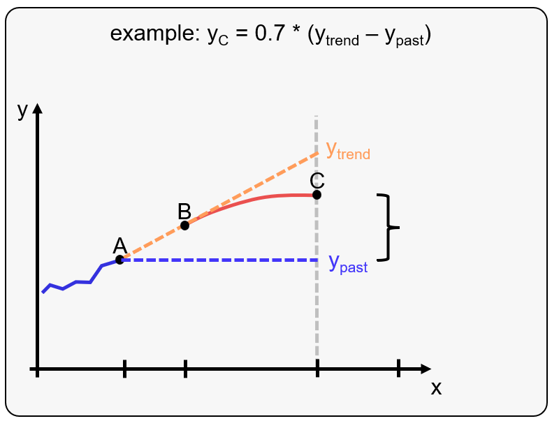
target point with data driven approach

For the temporal period both approaches are possible

• given values: a table with target values has to be provided (for each group, e.g. spatial unit and nationality).

• data-driven approach: the proportion of trend has to be selected (parameter e.g. 0.7)

The FSO uses three alternative modules for the temporal period:

module	description	values required
cubic	Interpolation from the start to the target point of the temporal period with a third-degree polynomial	temporal_model: “cubic” year_begin: first year of the cubic forecast year_end: last year of the cubic forecast trend_prop: proportion of trend to derive the target point; this has to be specified for the data driven approach temporal_end: given target points; has to be specified if given values for the end of the temporal period are used z0_prop: the Bézier function uses the slope at the starting point of the temporal period. This is calculated from the trend period model. The parameter z0_prop is the proportion of the calculated slope that is used as slope of the curve at the starting point. This parameter is responsible for the curve shape at the transition between the trend and the temporal period. z1_prop: the Bézier function also uses the slope at the end point of the temporal period. The parameter z1_prop is the proportion of the previously calculated slope (according to the trend model) that is used as slope of the curve at the end point. This parameter is responsible for the curve shape at the transition between the temporal and the constant period.
Bézier	Interpolation from the start to the target point of the temporal period with a Bézier-curve	temporal_model: “Bezier” year_begin: first year of the Bézier forecast year_end: last year of the Bézier forecast trend_prop: proportion of trend to derive the target point; has to be specified for the data driven approach temporal_end: given target points; has to be specified if given values for the end of the temporal period are used z0_prop: proportion of the slope at the starting point (same as for the cubic module) z1_prop: proportion of the slope at the end point (same as for the cubic module)
constant	The last value of the trend period is used for the temporal period	temporal_model: “constant” year_begin: first year of cubic forecast year_end: last year of cubic forecast

Constant period

For the last section of the TFR and MAB forecast the FSO uses a constant model.

module	description	values required
constant	The last value of the temporal period is used for the constant period	constant_model: “constant” year_begin: first year of the forecast year_end: last year of the forecast

Examples

Create input data

library(propopbirth)
library(ggplot2)
library(dplyr)

# load package data
data("fso_pop")
data("fso_birth")

Create input data

input <- create_input_data(
  population = fso_pop,
  births = fso_birth,
  year_first = 2011,
  year_last = 2023,
  age_fert_min = 15,
  age_fert_max = 49,
  fert_hist_years = 3,
  binational = TRUE
) 

Example 1

• topic: TFR forecast

• approach: given target points

• trend model: linear

• temporal model: cubic

Given target points (subjectively selected values)

temporal_end_tfr <- tidyr::expand_grid(
  spatial_unit = c("Aarau", "Frauenfeld", "Stadt Zürich"), 
  nat = c("ch", "int")) |> 
  dplyr::mutate(y_end = c(0.8, 1.5, 0.8, 2.0, 0.9, 0.9))

TFR forecast

forecast_tfr_example1 <- forecast_tfr_mab(
  topic = "tfr", 
  topic_data = input$tfr,
  trend_model = c(
    model = "lm", start = 2024, end = 2026, trend_past = 7, trend_prop = 0.5
  ),
  temporal_model = c(
    model = "cubic", start = 2027, end = 2055, trend_prop = 0.8, z0_prop = 0.7, 
    z1_prop = 0
  ),
  temporal_end = temporal_end_tfr,
  constant_model = c(model = "constant", start = 2056, end = 2075)
) 

ggplot(forecast_tfr_example1) +
  geom_line(aes(x = year, y = tfr, color = category)) +
  geom_point(aes(x = year, y = tfr, color = category)) +
  scale_color_manual(values = c("#ffe562", "#A05388", "#ffa81f", "#007AB8")) +
  labs(color = "Model", y = "TFR") +
  facet_wrap(nat ~ spatial_unit) +
  theme_bw()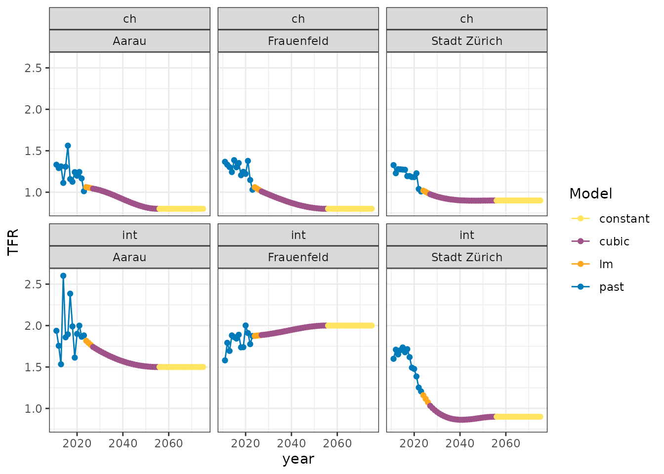

Example 2

• topic: TFR forecast

• approach: data-driven

• trend model: ARIMA

• temporal model: Bézier

forecast_tfr_example2 <- forecast_tfr_mab(
  topic = "tfr", 
  topic_data = input$tfr,
  trend_model = c(
    model = "ARIMA", start = 2024, end = 2026, trend_past = 7, trend_prop = 0.5
  ),
  temporal_model = c(
    model = "Bezier", start = 2027, end = 2055, trend_prop = 0.8, z0_prop = 0.7, 
    z1_prop = 0
  ),
  temporal_end = NA,
  constant_model = c(model = "constant", start = 2056, end = 2075)
  ) 
#> Registered S3 method overwritten by 'quantmod':
#>   method            from
#>   as.zoo.data.frame zoo

ggplot(forecast_tfr_example2) +
  geom_line(aes(x = year, y = tfr, color = category)) +
  geom_point(aes(x = year, y = tfr, color = category)) +
  scale_color_manual(values = c("#ffa81f", "#A05388", "#ffe562", "#007AB8")) +
  labs(color = "Model", y = "TFR") +
  facet_wrap(nat ~ spatial_unit) +
  theme_bw()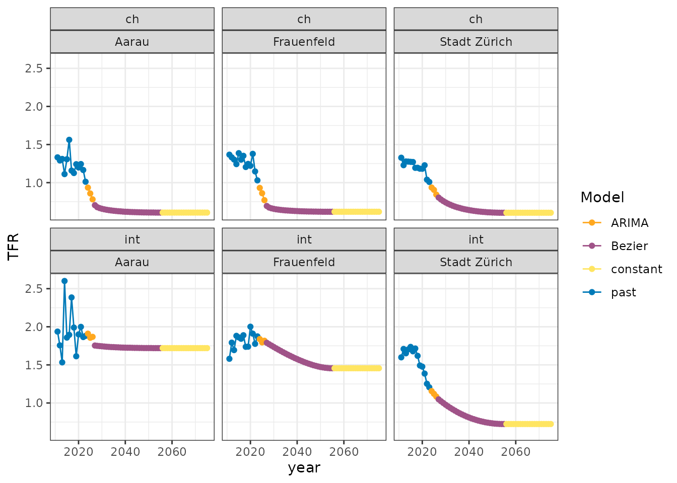

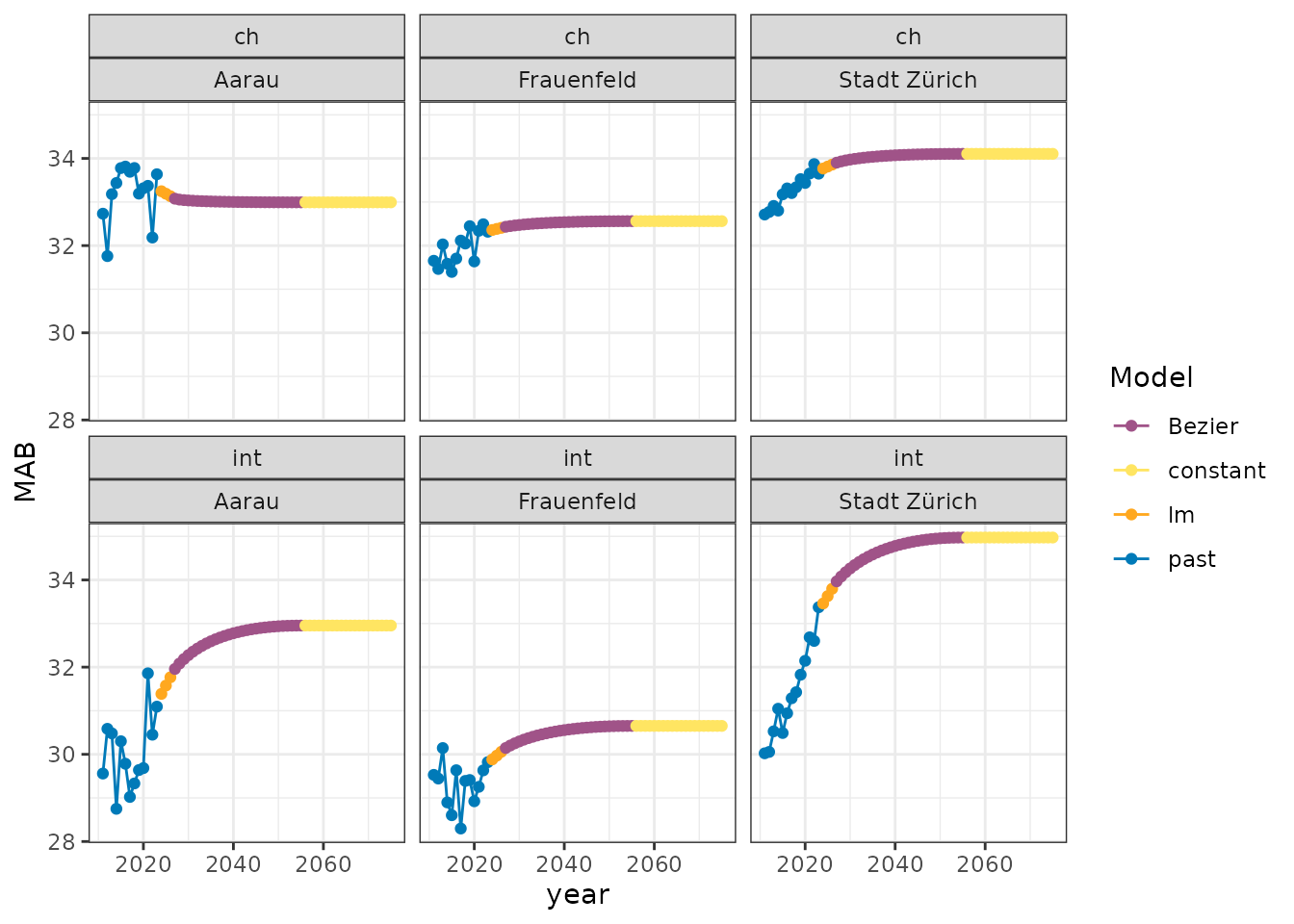
Example 3

• topic: MAB forecast

• approach: data-driven

• trend model: linear

• temporal model: Bézier

forecast_tfr_example3 <- forecast_tfr_mab(
  topic = "mab", 
  topic_data = input$mab,
  trend_model = c(
    model = "lm", start = 2024, end = 2026, trend_past = 7, trend_prop = 0.5
  ),
  temporal_model = c(
    model = "Bezier", start = 2027, end = 2055, trend_prop = 0.3, z0_prop = 0.7, 
    z1_prop = 0
  ),
  temporal_end = NA,
  constant_model = c(model = "constant", start = 2056, end = 2075)
) 

ggplot(forecast_tfr_example3) +
  geom_line(aes(x = year, y = mab, color = category)) +
  geom_point(aes(x = year, y = mab, color = category)) +
  scale_color_manual(values = c("#A05388", "#ffe562", "#ffa81f", "#007AB8")) +
  labs(color = "Model", y = "MAB") +
  facet_wrap(nat ~ spatial_unit) +
  theme_bw()